Causality, Confounding and Collider Bias
After spending some time learning more about causality over the past few months, here’s a learning summary post about key concepts behind causality as well as related topics to causal modelling. Before diving in, let’s start with the famous scene from the Matrix where Morpheus offers the red and blue pill to Neo.

What would you do knowing that you can only choose one, and only experience a single outcome without ever finding out what could have happened if you chose to take the other action? This philosophical question centered about choice actually lies deeply with causality itself. With that in mind, let’s begin with a primer on causality.
Simple causality primer
The idea behind causality is to identify the treatment effect (typically named as T) on an outcome response (typically named as Y). For example, if you had a headache, you would want to find out if taking a particular pill (T) would cure the headache (Y).
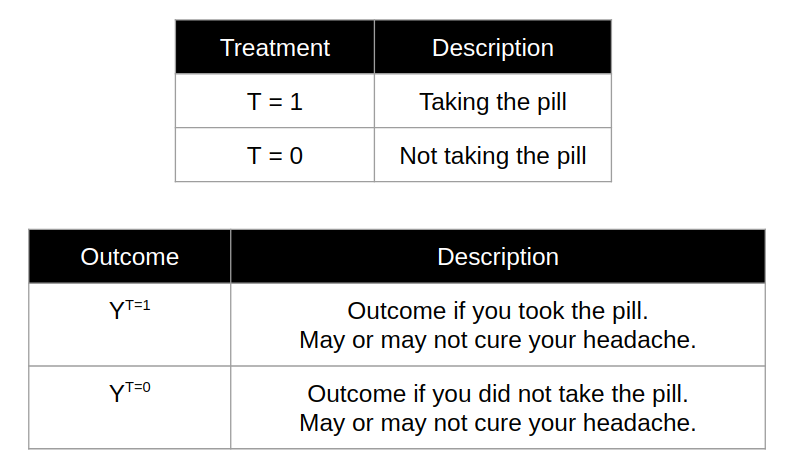
The fundamental problem of causal inference stems from the fact that you can only observe one outcome for a given single “unit”. A “unit” is used to refer to a specific experimental unit/iteration, which in this case refers to your particular experience of having the headache at that point in time. You can only choose to either:
- Take the pill [T = 1] or
- Not to take the pill [T = 0].
Consequently, you get to observe the outcome from your chosen treatment (Y_t | T = t, where t represents 1 or 0), but not the outcome of the treatment that you did not choose to take. The latter is known as the counterfactual, which represents the outcome of “what would have happened”. To tackle this fundamental problem, one would have to refer to the potential outcomes causal model framework by Rubin, whereby you need to make assumptions to estimate the missing counterfacual.
In the example above, suppose you decide to take the pill. Thus, you would have observed the outcome for Y_1 | T = 1, but you would not have observed the counterfactual outcome for not taking the pill Y_0 | T = 0. At an individual level, it will be impossible to obtain the counterfactual outcome, and thus it is impossible to calculate the individual treatment effect as measured by the difference in observed outcome versus counterfactual outcome.
By conducting experiments at a population level, we can calculate the average treatment effect. As shown by in the following table, we have 8 participants where 4 of them having T = 1 vs 4 of them having T = 0. The counterfactual outcome for each individual is represented by the question mark.
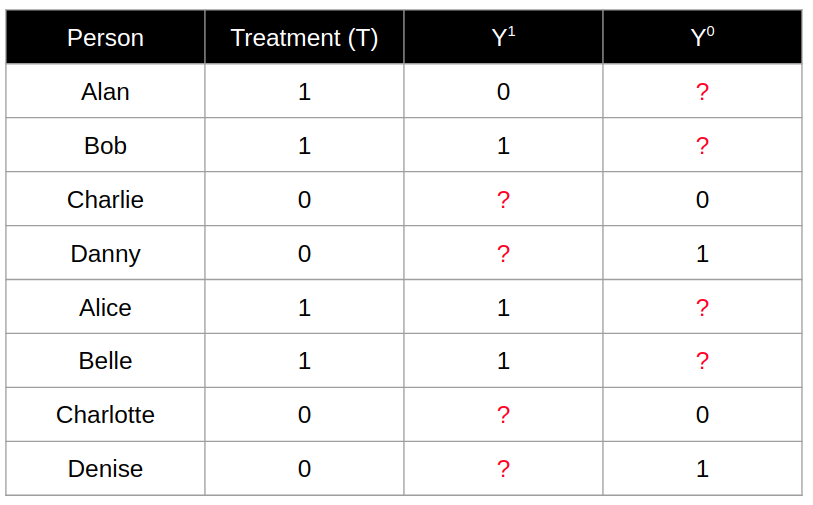
What is intuitive or commonsensical is that in the above example, we can calculate the average treatment effect as E(Y_1 - Y_0) = 3/4 - 2/4 = 0.25. To arrive at that conclusion, we made some assumptions to identify the causal effects such that it can be mathematically calculated as a difference between outcomes of the different treatment groups.
Assumptions behind identifiability of causal effects
The identifiability of causal effects requires making some untestable assumptions called causal assumptions:
Stable Unit Treatment Value Assumption (SUTVA)
As a concept, SUTVA involves two implicit assumptions:
- Units do not interfere with each other. In other words, the treatment assignment of one unit does not affect the OUTCOME of another unit.
- There is only one version of treatment that is consistent across all units.
Consistency
The consistency assumption states that the potential outcome under treatment T = t, Y^t is equal to the observed outcome if the actual treatment received is T = t.
Positivity
The positivity assumption states that for every set of values for X covariates, treatment assignment was not deterministic.

If this was violated, it will mean that for a given value of X, everybody is either treated or not treated at all. Within that level of X, it would be impossible to learn the causal treatment effect.
Suppose that for some values of X, the treatment assignment was deterministic as represented by the following example where there is no control group (T = 0):

then we would have no observed outcome values of Y for the control group for those values of X.
Ignorability
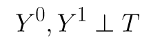
This is also known as the no unmeasured confounders assumption. In mathematical form, the potential outcomes are independent from the treatment assignment.
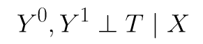
Under situations where you have additional covariates commonly represented by X, it represents the conditional independence of treatment assignment from potential outcomes.
Ignorability is the key assumption that allows us to use the outcomes from different units under different treatment as the corresponding counterfactuals outcomes, and thus “populate” the “?” marks that we saw in a previous example. The concept stems from the idea that given the right covariates, treatment itself becomes ignorable.
Revisiting the previous example of an experiment conducted on 8 participants, we also expanded the table by including the Gender as a covariate X.
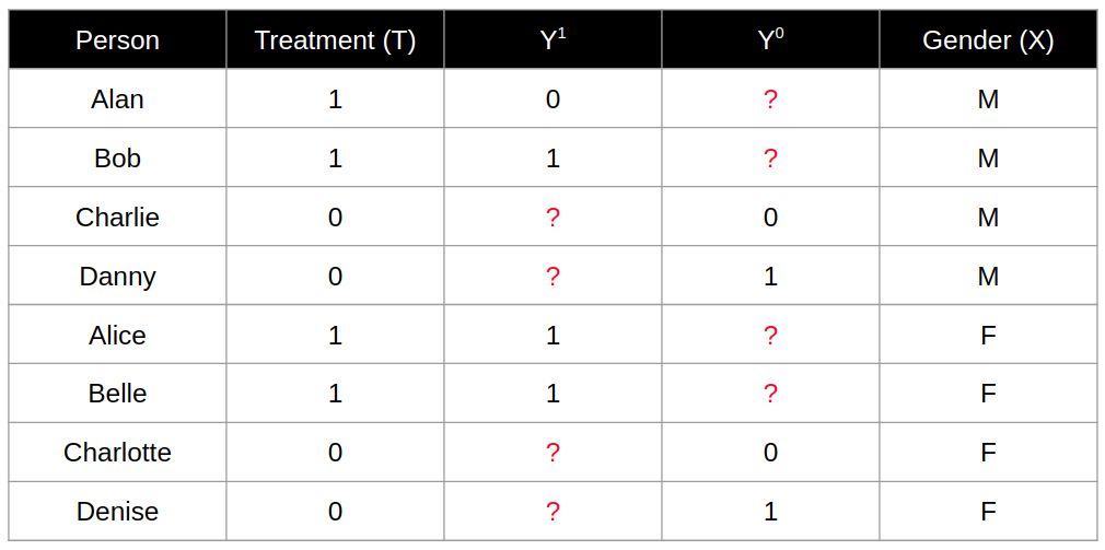
In this example, we have great balance across different values of X. Both genders (Male or Female) have 4 experimental units each, with 2 the in treatment group and 2 in the control group.
With the presence of the covariate X, we can determine the conditional average treatment effect (CATE) which is determining the average treatment effect within different subpopulations out of the general population. With respect to the example, we have the following calculations:
CATE for Males = E(Y1 - Y2 | X = M) = (1/2) - (1/2) = 0.5 - 0.5 = 0
CATE for Females = E(Y1 - Y2 | X = F) = (2/2) - (1/2) = 1 - 0.5 = 0.5
Confounding in causality
To understand how confounding comes into play within causality, we can take a look at a system that has 3 variables, where X represents the confounder. This can be represented by the graphical model shown below, where the nodes represent the variables and the directed edges represent the relationship with a causal direction.
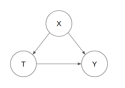
Note that this graph is a representation of a directed acyclic graph (DAG) where:
- All the edges between nodes have direction
- There is no cyclicity in the causal relationship between nodes.
As shown, the confounder affects both the treatment variable T and response variable Y. An example of this could be X as Age, T as Physical Activity, Y as Mortality. In this hypothetical example, when one is younger, you tend to have greater physical activity and at the same time, your immune system is stronger. As you get older, you tend to have less physical activity and at the same time, your mortality increases perhaps due to a weakening immune system.
Thus, the direct causal relationship between physical activity as a treatment variable on the outcome variable mortality may not be easily identifiable since there is the confounding variable that affects both the treatment variable and outcome.
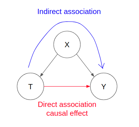
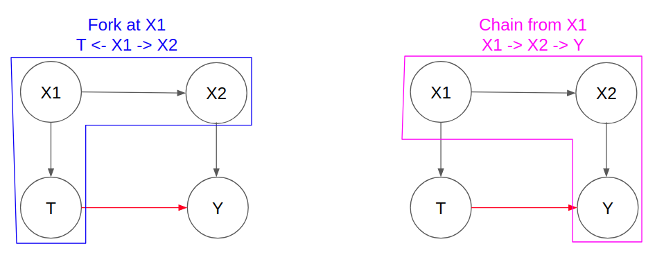
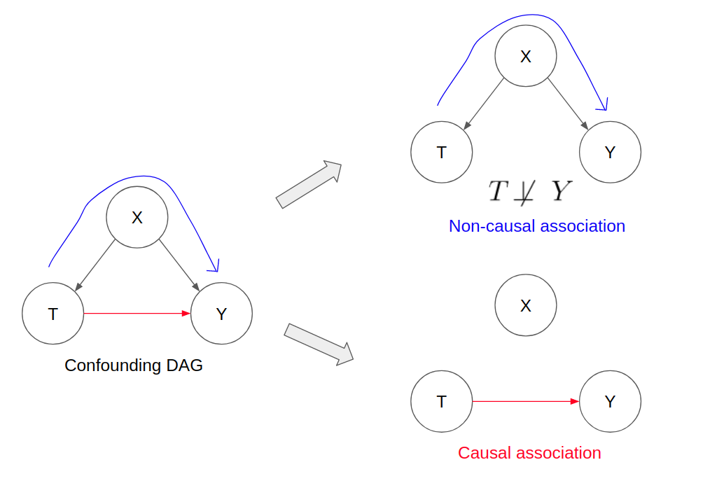
When we speak about causality, we want to identify the direct causal association between the treatment variable on the outcome variable (as shown by the red arrow). In the context of confounding variables, there is always indirect association that runs through the confounder variable (as shown by the blue arrow). Note that this is a simplified graph, but this can be extended to other graphs where X itself is a series of nodes that represent forks or chains.
To understand how the indirect non-causal association comes into play, we need to understand the concept of independence and conditional independence for different graphical models.
Independence and conditional independence of variables
When variables are independent of each other, that means that knowing one variable does not change the probability of determining the other. In other words, for two independent variables A and B,

Conditional independence between two variables A and B involve extra variables to be conditioned on. For two variables A and B that are conditionally independent on variable C,
For graphical relationships represented by Forks and Chains, we observe:
- Conditional independence between the “side” nodes if we condition upon the “center” variable (shown by the shading). This is also known as “blocking” the dependence association between the “side” nodes.
- Both “side” variables are not independent by themselves.
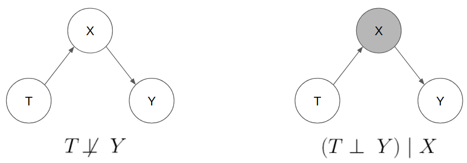
In a Fork that stems from X and branches out to T and Y (T <- X -> Y), we observe the following:
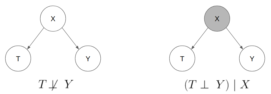
An example of a Fork situation can be exemplified by rainy weather (represented by X in the graph above) versus the number of vehicle accidents and number of cold flu cases (represented by T and Y).
- By themselves, Y and T are not independent on each other. When there is heavy rain (X) but assuming we did not know X, we may observe higher counts of vehicle accidents (T) and cold flu cases (Y) and thus there will be some correlation between them. Thus, knowing T will help us know more about Y, and vice versa.
- By conditioning on rainy weather X, knowing the count of vehicles accidents T does not help you to gain more information about the number of cold flue cases Y. In other words,
P(Y|T,X) = P(Y|X)
In a Chain that stems from T to X to Y (T -> X -> Y), we observe the following:
An example of a Chain situation can be exemplified by a genetic disease along an ancestry line where in this case (T -> X -> Y), T is the grandparent, X is the parent, and Y is the child.
- By themselves, Y and T will demonstrate dependence between each other. If T has the disease, it is also likely that Y has the disease. If T does not have the disease, it is also likely that Y does not have the disease.
- By conditioning on the middle node X (or knowing what X has), knowing if T has the disease does not help you to gain more information about Y having the disease. In other words,
P(Y|T,X) = P(Y|X)
For a graphical relationships represented by Colliders, we observe:
- Independence between the “side” nodes WITHOUT conditioning upon the “center”/”collider” variable.
- Conditioning upon the “collider” variable (shown by the shading) will open up a dependence association between the “side” variables
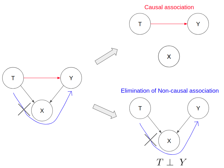
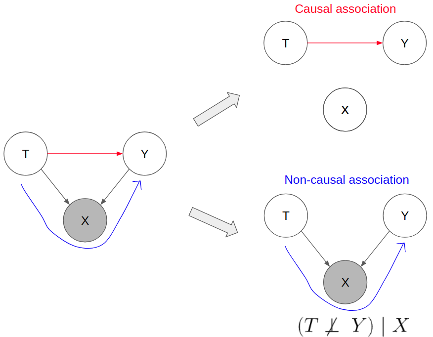
In a Collider that collides at X from T and Y (T -> X <- Y), we observe the following:
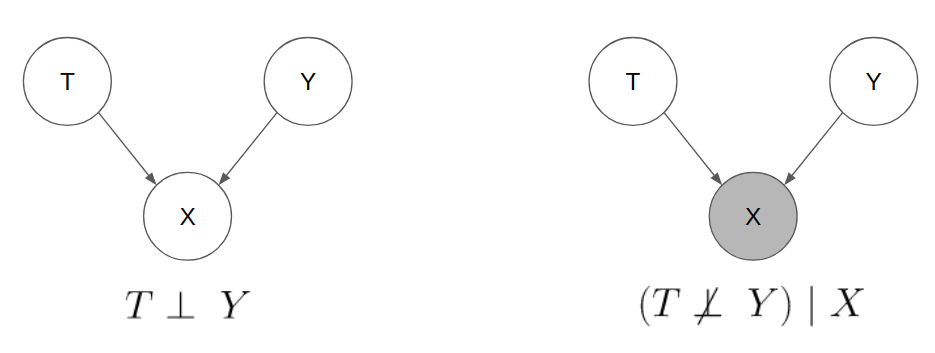
An example of a Collider situation is the eye colour of parents (represented by T and Y in the graph above) versus the eye colour of their child (represented by X). Suppose that in this hypothetical world, having green eye colour is a dominant trait.
- The eye colour of the parents (T and Y) by themselves are independent of each other.
- By conditioning on the eye colour of the child (X), the eye colour of both parents (T and Y) become conditionally dependent.
- If the child has green eye colour and one parent does not have green eye colour, we can conclude that the other parent must have green eye colour.
- If the child does not have green eye colour and one parent does not have green eye colour, we can conclude that the other parent must not have green eye colour.
Interventional versus observational distributions
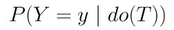
To identify the causal effect of treatment, we need to understand the idea of interventional distributions. Intervention of the treatment variable T implies taking the whole population and subjecting them to the treatment effect. This can be represented by the “do” operator as shown by the following equation, where Y represents the potential outcome:
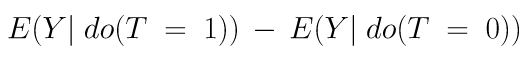
Based on this framework, the average treatment effect (ATE) is represented by the following causal estimand.
Note that the idea of interventional distributions is not the same as observational distributions (which do not have the “do” operator). In observational distributions, we deal with “conditioning” that splits the population into subpopulations while in interventional distributions, we deal with “do” interventions that compares population with similar attributes. This is shown in the diagram as taken from “Introduction to Causal Inference” textbook by Brady Neal.
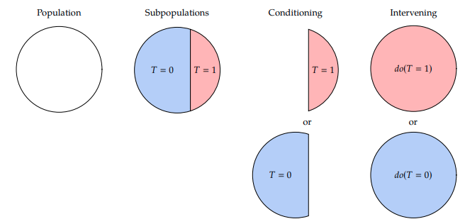
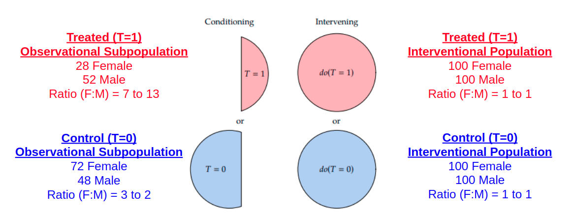
The key difference between interventional distribution and observational distributions is that the covariate distribution between the different subpopulations may not be the same. Recall that we are interested in the average treatment effect among the whole population.
- In interventional distributions, we are comparing the difference in outcomes between populations that have similar attributes/covariates, and thus it is a fair comparison of treatment effects.
- In observational distributions, this may not necessarily be the same since there might be a confounder that distorts the Treatment assignment among the subpopulations. For example, perhaps Gender (as a confounder) may affect the treatment assignment such that there is a higher proportion of males in the Treated subpopulation while there is a higher proportion of females in Control subpopulation. Thus, we cannot simply find the difference in response outcomes between the treated and control population since they do not have the same breakdown.
Also, interventional distributions (with “do” operators) are used for causal estimands while observational distributions (without any “do” operators) are used for statistical estimands. This might be slightly technical but here’s a proposed framework (taken from the “Introduction to Causal Inference” textbook by Brady Neal) which is shown in the following visualisation:
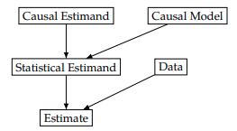
For causal modelling, we want to estimate causal estimands. This can be done with either:
- interventional distributions (available by experimental data) or
- reducing the causal estimands into statistical estimands by applying an appropriate “causal model”.
Subsequently, to estimate the statistical estimands, we can use available observational data, and perform the correct adjustments with it depending on the “causal model”. In the next section, we will explore simple examples of the “adjustments” required for different types of causal models.
Causal estimand identification with observational data under different causal models
In this section, we will take a look at the various adjustments that are needed in order to utilise observational data with the appropriate causal model. Note that the key assumptions remain (SUTVA, consistency, ignorability, positivity) still apply since we are trying to identify a causal estimand.
Causal model with confounding variables
In the simple example where X is a confounding variable that affects T and Y, there is direct causal association flowing from T to Y and indirect non-causal association flowing from T to X to Y (as represented by the fork graphical representation which implies T and Y are not independent).
Since we are only interested in the direct causal association, this relates back to the idea of interventional distributions. In interventional distributions, we seek to set the treatment variable as a specific value in order to observe the treatment effect on the outcome variable. This implies that all edges that are incoming into T are eliminated.
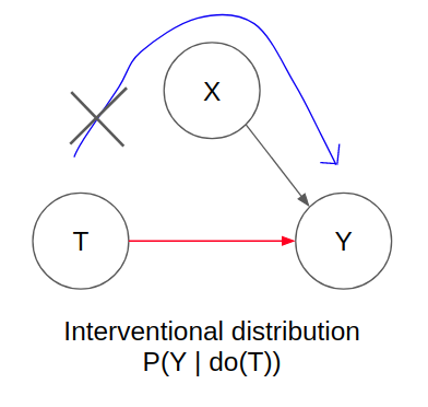
This is only achievable either through:
- Experiments where the treatment assignment is randomised (thus breaking down the confounding relationship between X and T)
- Observational data where there is no indirect non-causal association flowing.
In the second option, with observational data, we can use what we understand about conditional independence with Forks. We can condition on X which breaks the non-causal association between T and Y. This effectively reduces the diagram to one that only has the direct causal association flowing between T and Y. This is also known as the backdoor adjustment criteria but I won’t go into greater detail as it requires much more indepth explanations about d-separation.
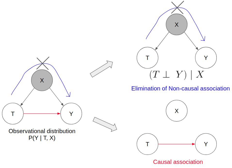
As shown, this observational distribution (without any “do” operators) is the equivalent of the interventional distribution (with “do” operators).
Thus, it is through this identification process that the causal estimand of the ATE can be identified through a statistical estimand, which can subsequently be estimated through observational data.
Causal model with collider variables
If the causal model diagram has a collider variable X between T and Y, we have to be careful in terms of how to use observational data to identify the causal estimand. Likewise, we can use what we understand about Colliders to establish the independence between T and Y.
If we condition on the collider variable X, it will open up a path of indirect non-causal association between T and Y. Estimation of the treatment effect by conditioning on X will lead to collider bias.
Summary
In this blog post, I have provided a summarised walkthrough about some introductory concepts about causal inference (including confounding, graphical models, independence, conditional independence, etc) and how to identify the ATE/CATE through observational data under various causal models.
In the next blog post, I will work through some R code and simulation examples to illustrate how we can use observational data to estimate the treatment effect under the appropriate causal model relationships.